DS250 - UW Intro to Data Science Course Project
Background
This was my course project in Introduction to Data Science, the first course in a three-course certificate program through the University of Washington.
I’m publishing it here, warts and all, because I think there are a few interesting facets to the analysis.
- Flexing my metaphorical mapping and visualization bicep with GGPLOT and GGMAP
- A first foray / experiment into using Principal Component Analysis (PCA)
- Leveraging multiple models - a decision tree for feature selection, PCA to address multicollinearity, and a linear regression to predict graduation rate
- A stark lesson in how hard it is to make sexy infographics!
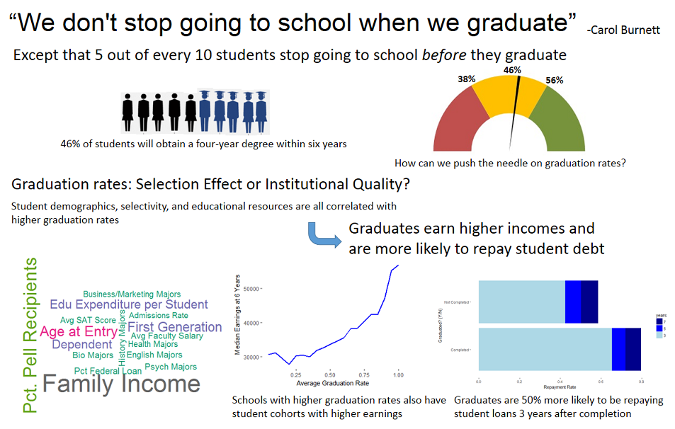
- Surprising results - I was surprised that measures of family income are so highly correlated with both average SAT score and colleges’ graduation rates. What are the implications for education policy?
College Scorecard Analytics Project
A study of colleges in the US has collected information regarding school and student demographics, degrees awarded by subject area as well as financial information including average degree cost by income bracket, student tuition and scholarships, repayment rates, and post-college average earnings.
Exploratory data analysis
0 Where are the colleges located?
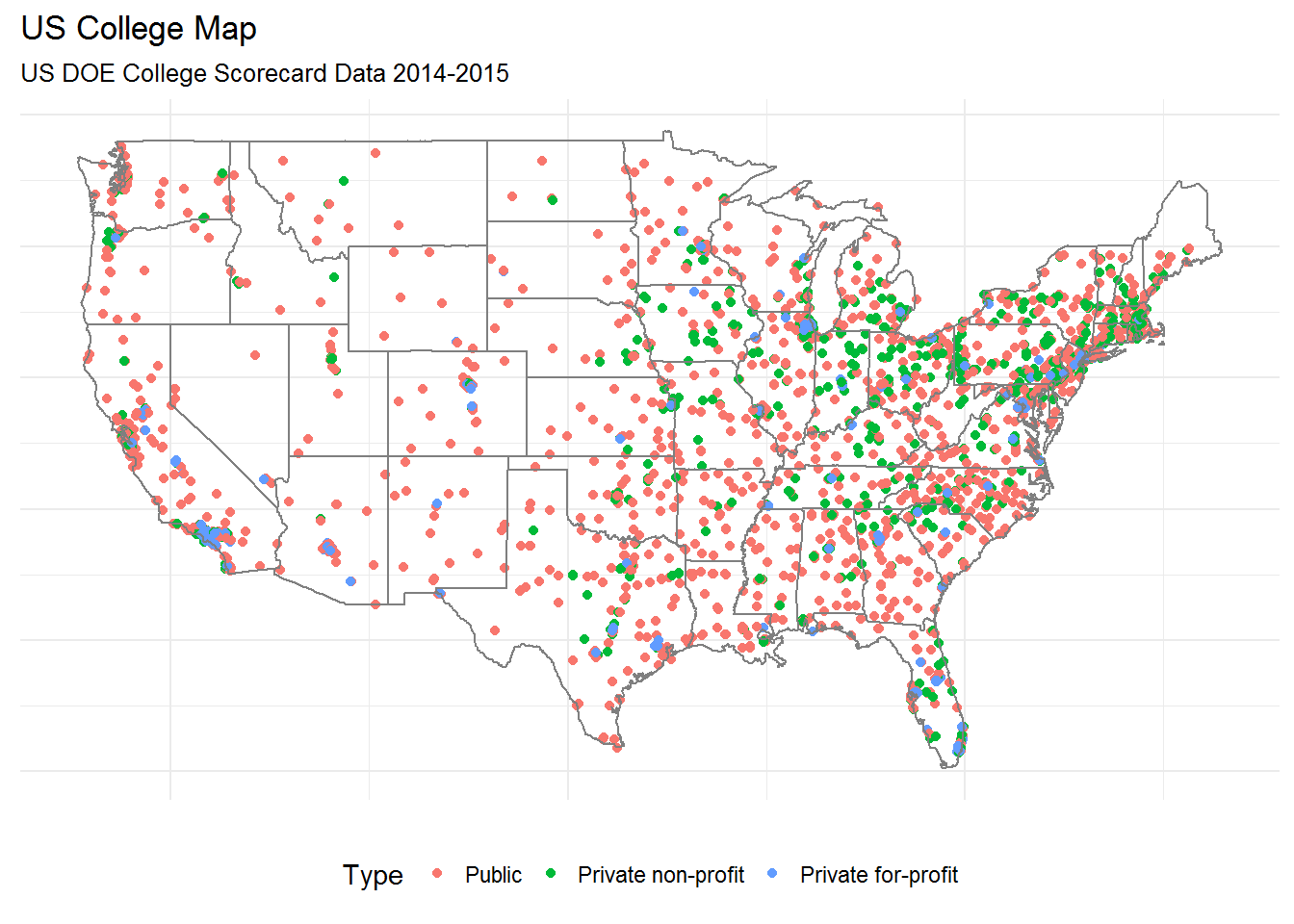
US colleges appear to be distributed similarly to the overall US population.
Among college types, however, it appears that Public colleges are the most likely to be located in rural areas, while Private for-profit colleges are primarily centered around urban areas.
This is particularly noticeable given that there are nearly twice as many private for-profit colleges as public colleges:
## # A tibble: 3 x 3
##   CONTROL `n()`               type
##     <int> <int>              <chr>
## 1       1  2044             Public
## 2       2  1956 Private non-profit
## 3 3 3703 Private for-profit2.1. Count of colleges by degree length and region
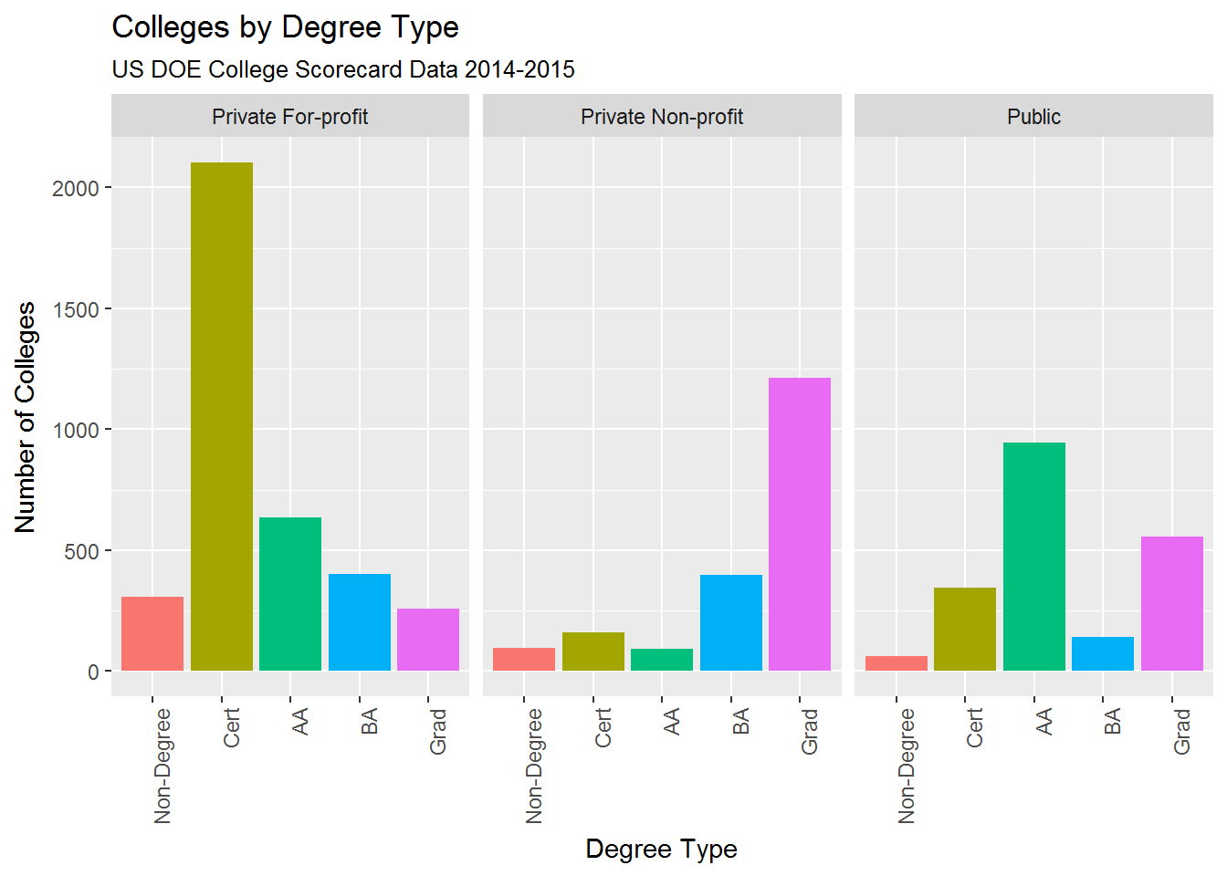
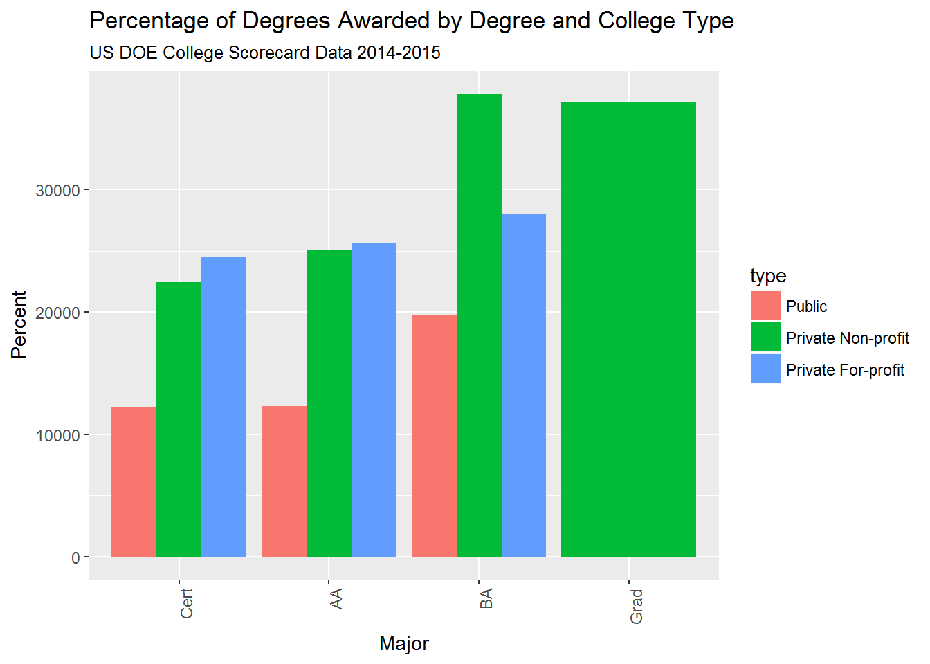
College ownership appears related to the degree-type awarded:
- The bulk of Private for-profit colleges are certificate-granting
- Public community colleges (Associates degree-granting) outnumber Public four-year institutions
- Private non-profit colleges specialize in undergraduate and graduate degrees
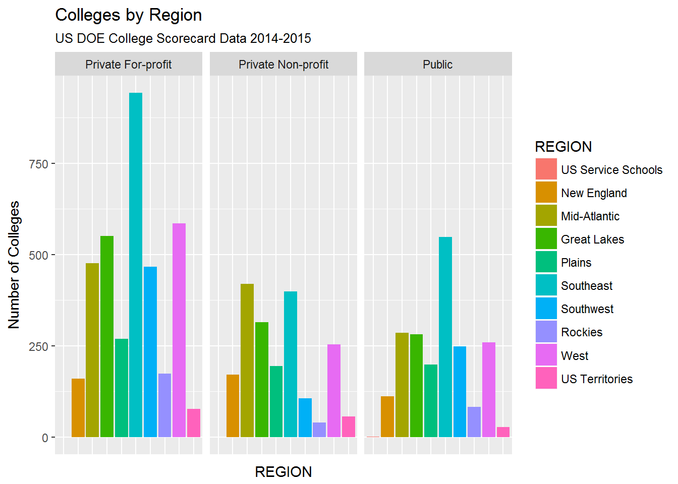
I’m not sure what conclusions we can draw about regional distribution of colleges, beyond the fact that the Southeast appears overrepresented. Deeper analysis should adjust college counts by total population to compare the number of colleges per capita.
2.2. Categorize student graduation counts by degree name
Health, business/marketing, cuinary, and humanities are all top majors:
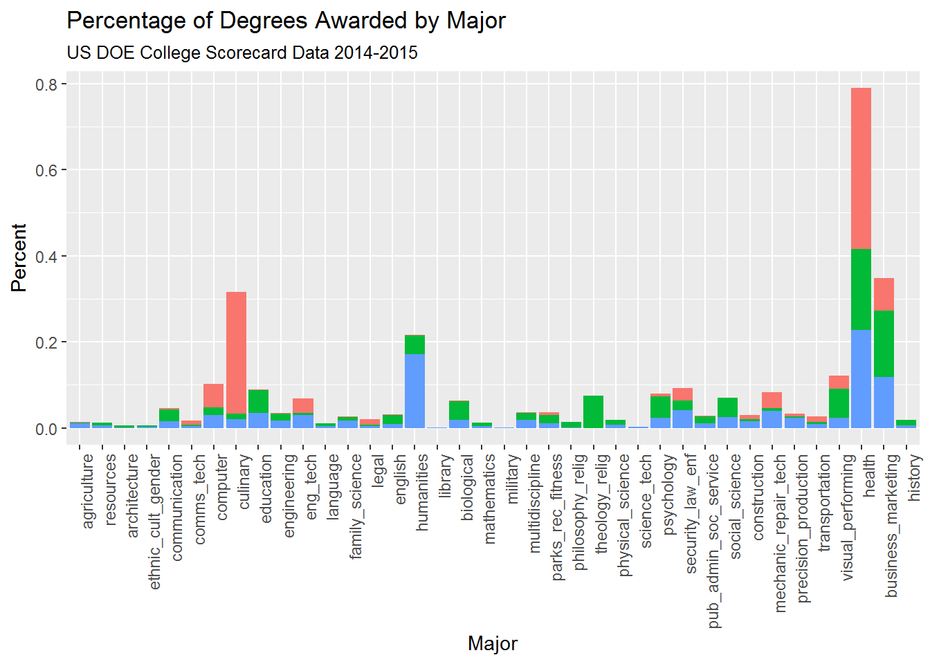
Top 5 majors by college type:
#public
t.major2[t.major2$Type=="Public",][1:5,]
## Type variable value
## 106 Public health 0.22663601
## 46 Public humanities 0.17144393
## 109 Public business_marketing 0.11892869
## 82 Public security_law_enf 0.04044814
## 94 Public mechanic_repair_tech 0.03918093#private non-prof
t.major2[t.major2$Type=="Private Non-Profit",][1:5,]## Type variable value
## 107 Private Non-Profit health 0.18948482
## 110 Private Non-Profit business_marketing 0.15411169
## 71 Private Non-Profit theology_relig 0.07446778
## 104 Private Non-Profit visual_performing 0.06753585
## 26 Private Non-Profit education 0.05250905#private for-prof
t.major2[t.major2$Type=="Private For-profit",][1:5,]## Type variable value
## 108 Private For-profit health 0.37294668
## 24 Private For-profit culinary 0.28278959
## 111 Private For-profit business_marketing 0.07457577
## 21 Private For-profit computer 0.05469259
## 96 Private For-profit mechanic_repair_tech 0.03740514Private for-profit schools are the main providers of culinary programs, while private non-profit colleges specialize in theology/religious studies (likely religiously-affiliated colleges) and the visual and performing arts.
Study Evaluation
3.1. Study type, experimental model, and approach
The College Scorecard (https://collegescorecard.ed.gov/data/) is a collection of data on US colleges regarding school and student demographics, degrees awarded by subject area, as well as financial information including average degree cost by income bracket, student tuition and scholarships, repayment rates, and post-college earnings.
Data are self-reported and observational (there are no tests or treatments being applied).
Experimental design:
- Predict each college’s graduation rate (completion of a 4-year degree within 6 years)
- Response variable, graduation rate, is a numeric attribute with a range of [0,1]
- My approach is to use data from the 2013/14 academic year (year t-1) to predict graduation rates in the subsequent year, the 2014-15 academic year (year t)
- Features will be generated from the College Scorecard data set and include numeric and categorical attributes
3.2. Bias
- Data exclude part-time students
- Data are self-reported. There is potential response bias because only schools that are good performers are incentivized to provide information
- Evaluation of graduation rates is focused on completing a 4-year degree, when most students don’t do a Bachelor’s, they do trade school or associate’s degree. In general, performance criteria might be more geared towards 4-year degree holders than community colleges.
3.3. Hypothesis
School selectivity - as measured by admissions rate and average SAT score - is positively correlated with graduation rate.
School ownership (Public/Private non-profit/Private for-profit) is correlated with graduation rate. Specifically, private non-profits have the highest graduation rate, followed by public colleges followed by private for-profit colleges.
Graduation rates are highest for graduate students, followed by Bachelor’s, Associate’s, and certificates.
Summary analysis - Value-add analysis for education
4.0. Cost by College Type
Private non-profit colleges are more than twice as expensive as Public colleges and nearly 40% more expensive than Private for-profit colleges.
## # A tibble: 3 x 2
##                 type avg_cost
##                <chr>    <dbl>
## 1             Public 14922.46
## 2 Private Non-profit 35607.98
## 3 Private For-profit 25902.304.1. Cost by Degree
Most of the cost differential between Private non-profit and for-profit colleges is due to the face that Bachelor’s and graduate degrees at Private non-profit schools are significantly more expensive than at Private for-profits.
Surprisingly, there is not a large cost increase at Private for-profits as you go from certificate degrees to Associate’s and Bachelor’s.
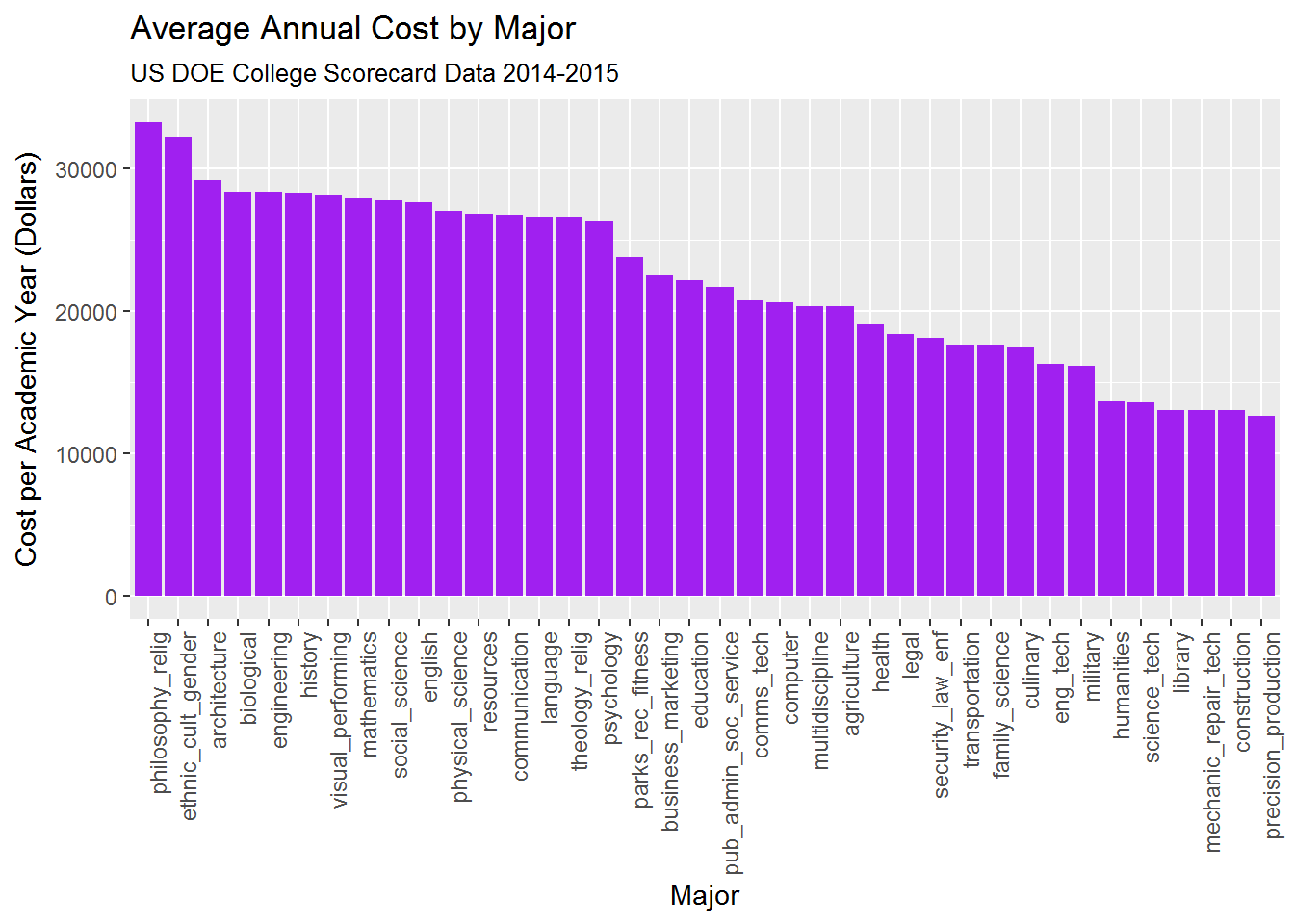
4.1a. Cost by Major
The most expensive majors cost 2-3x the least expensive. The most expensive majors are those most-commonly awarded at Private colleges (Philosophy, Religion, Ethnic/Cutlural/Gender studies, Architecture), while the least-expensive majors are associated with skilled trades (Mechanic/Repair/Technician, Construction, and Precision Production).
4.2. Cost by College
The most expensive colleges are all Private non-profit schools, mostly located in major metropolitan areas. Community colleges are the most affordable, whereas if you want to attend a low-cost Private college, head to the Caribbean!
Top 5 most expensive colleges
##                                        INSTNM COSTT4_A
## 1                       University of Chicago    64988
## 2 Columbia University in the City of New York    64144
## 3                      Sarah Lawrence College    64056
## 4           Washington University in St Louis    63755
## 5                          Occidental College    63363
Top 5 least expensive colleges
##                              INSTNM COSTT4_A
## 1       Cleveland Community College     5536
## 2 Colegio Universitario de San Juan     5920
## 3     Pearl River Community College     6171
## 4         Harford Community College     6336
## 5               South Texas College     6374
Top 5 least expensive Private non-profit schools
##                                                   INSTNM COSTT4_A
## 1                           Caribbean University-Bayamon     8180
## 2                             Caribbean University-Ponce     8438
## 3 Pontifical Catholic University of Puerto Rico-Mayaguez     8716
## 4                            Atlantic University College     9521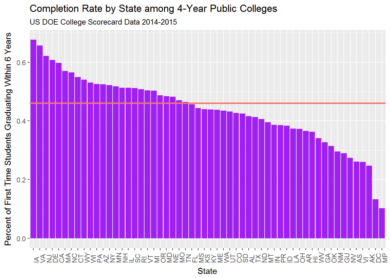
## 5 Dewey University-Hato Rey 100214.3. College completion rates by state, compared to national average
Predictive Model
Target = predict student graduation rate Train model on year T-1 (2013/2014 data) and evaluate predictions accuracy in year T (2014/2015 data)
5.1. Evaluate the primary features that affect college program completion
I chose to start with a regression tree to give first impressions of the key predictors of colleges’ graduation rates.
#Add additional predictors to the "scorecard" dataset used for data exploration
new.vars <- c('RELAFFIL','ADM_RATE','SAT_AVG','INEXPFTE','AVGFACSAL',
              'PFTFAC','PCTPELL','AGE_ENTRY','HCM2','MAIN','CCBASIC',
              'CCUGPROF','CCSIZSET','PCTFLOAN','FEMALE','MARRIED',
              'DEPENDENT','VETERAN','FIRST_GEN','ICLEVEL','FAMINC')

data14 <- cbind(scorecard,df_14_15[,new.vars])

#delete obs with missing target variable
data14 <- data14[!is.na(data14$C150_4),]

#import training data (2013/14 data)
df_13_14 <- as.data.frame(fread("C:/Users/nadav.rindler/OneDrive - American Red Cross/Training/UW Data Science Certificate/DS250/Course Project/CollegeScorecard_Raw_Data/MERGED2013_14_PP.csv",
                                na.strings=c("NULL","PrivacySuppressed")))
#fix UNITID name
colnames(df_13_14)[1] <- c("UNITID")

#training data
data13 <- df_13_14[!is.na(df_13_14$C150_4),which(names(df_13_14) %in% colnames(data14))]

#Regression Tree
library(rpart)
library(rpart.plot)

#check null values - some attributes are entirely null
null_list <- colSums(is.na(data13), na.rm=FALSE)
nulls <- null_list[null_list>0]
nulls
## HCM2 LOCALE CCBASIC CCUGPROF CCSIZSET RELAFFIL ADM_RATE
## 2448 2448 2448 2448 2448 2448 651
## SAT_AVG PCIP01 PCIP03 PCIP04 PCIP05 PCIP09 PCIP10
## 1069 1 1 1 1 1 1
## PCIP11 PCIP12 PCIP13 PCIP14 PCIP15 PCIP16 PCIP19
## 1 1 1 1 1 1 1
## PCIP22 PCIP23 PCIP24 PCIP25 PCIP26 PCIP27 PCIP29
## 1 1 1 1 1 1 1
## PCIP30 PCIP31 PCIP38 PCIP39 PCIP40 PCIP41 PCIP42
## 1 1 1 1 1 1 1
## PCIP43 PCIP44 PCIP45 PCIP46 PCIP47 PCIP48 PCIP49
## 1 1 1 1 1 1 1
## PCIP50 PCIP51 PCIP52 PCIP54 COSTT4_A AVGFACSAL PFTFAC
## 1 1 1 1 60 18 183
## PCTPELL PCTFLOAN AGE_ENTRY FEMALE MARRIED DEPENDENT VETERAN
## 2 2 12 118 379 144 1319
## FIRST_GEN FAMINC
## 170 12#convert some numeric values to factor
data13$CONTROL <- as.factor(data13$CONTROL)
data13$REGION <- as.factor(data13$REGION)
data13$ICLEVEL <- as.factor(data13$ICLEVEL)
data14$CONTROL <- as.factor(data14$CONTROL)
data14$REGION <- as.factor(data14$REGION)
data14$ICLEVEL <- as.factor(data14$ICLEVEL)
#data transformations
data13$INEXPFTE_exp <- exp(data13$INEXPFTE)
data14$INEXPFTE_exp <- exp(data14$INEXPFTE)
#religious affiliation doesn't exist in 2013 data. Join from 2014 data
#create an indicator variable to identify ANY religiously-affiliated college
data13 <- data13 %>%
select(-RELAFFIL) %>%
left_join(data14[,c("UNITID","RELAFFIL")], by="UNITID") %>%
mutate(RELAFFIL_IND=ifelse(RELAFFIL>=0,1,0))
data14$RELAFFIL_IND <- ifelse(data14$RELAFFIL>=0,1,0)
#remove from predictors - target var, ID vars, null vars
exclude <- c("C150_4","UNITID","INSTNM","HCM2","LOCALE","CCBASIC","CCUGPROF",
"CCSIZSET","RELAFFIL","LNFAMINC","STABBR","COSTT4_A")
varnames <- names(data13)[-which(names(data13) %in% exclude)]
fmla <- as.formula(paste("C150_4 ~ ", paste(varnames, collapse= "+")))
#Train tree
grad.tree <- rpart(fmla,data = data13, method="anova",
control=rpart.control(cp=0.001)) #increase model complexity over default (cp=0.01)
#prune tree to node with min xerror
p.grad.tree <- prune(grad.tree, cp=grad.tree$cptable[which.min(grad.tree$cptable[,"xerror"]),"CP"])
#plot tree
prp(p.grad.tree,faclen=2,varlen=20,cex=0.5)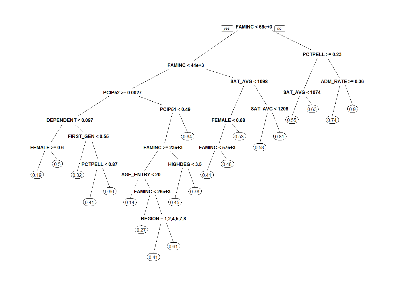
I’m surprised that the most important predictors of a college’s graduation rate relate to its students’ family incomes. Family income (FAMINC), percentage of the student body on Pell Grants (PCTPELL), average age at college entry (AGE_ENTRY), percentage of first generation students (FIRST_GEN), percentage of dependent students (DEPENDENT), and percentage of students on federal loans (PCTFLOAN) are all measures of the demographics and socioeconomic background of the student body.*
There are also several important predictors related to average SAT score and educational resources (instructional expenditure per student, INEXPFTE, and average faculty salary, AVGFACSAL)
*Note: Demographic data such as family income, etc. come from the National Student Loan Data System (NSLDS) which is pulling the data from students’ FAFSA forms.
#variable importance
importance <- as.data.frame(sort(p.grad.tree$variable.importance,decreasing=TRUE))
colnames(importance) <- "importance"
head(importance, n=10)
## importance
## FAMINC 49.833834
## PCTPELL 31.222093
## AGE_ENTRY 19.237627
## FIRST_GEN 18.525942
## INEXPFTE 14.680300
## DEPENDENT 14.319560
## PCTFLOAN 5.376605
## SAT_AVG 3.735139
## AVGFACSAL 3.725172
## PCIP54 3.247551Let’s visualize some of these relationships: 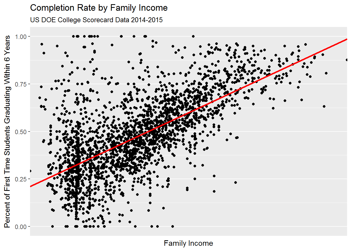
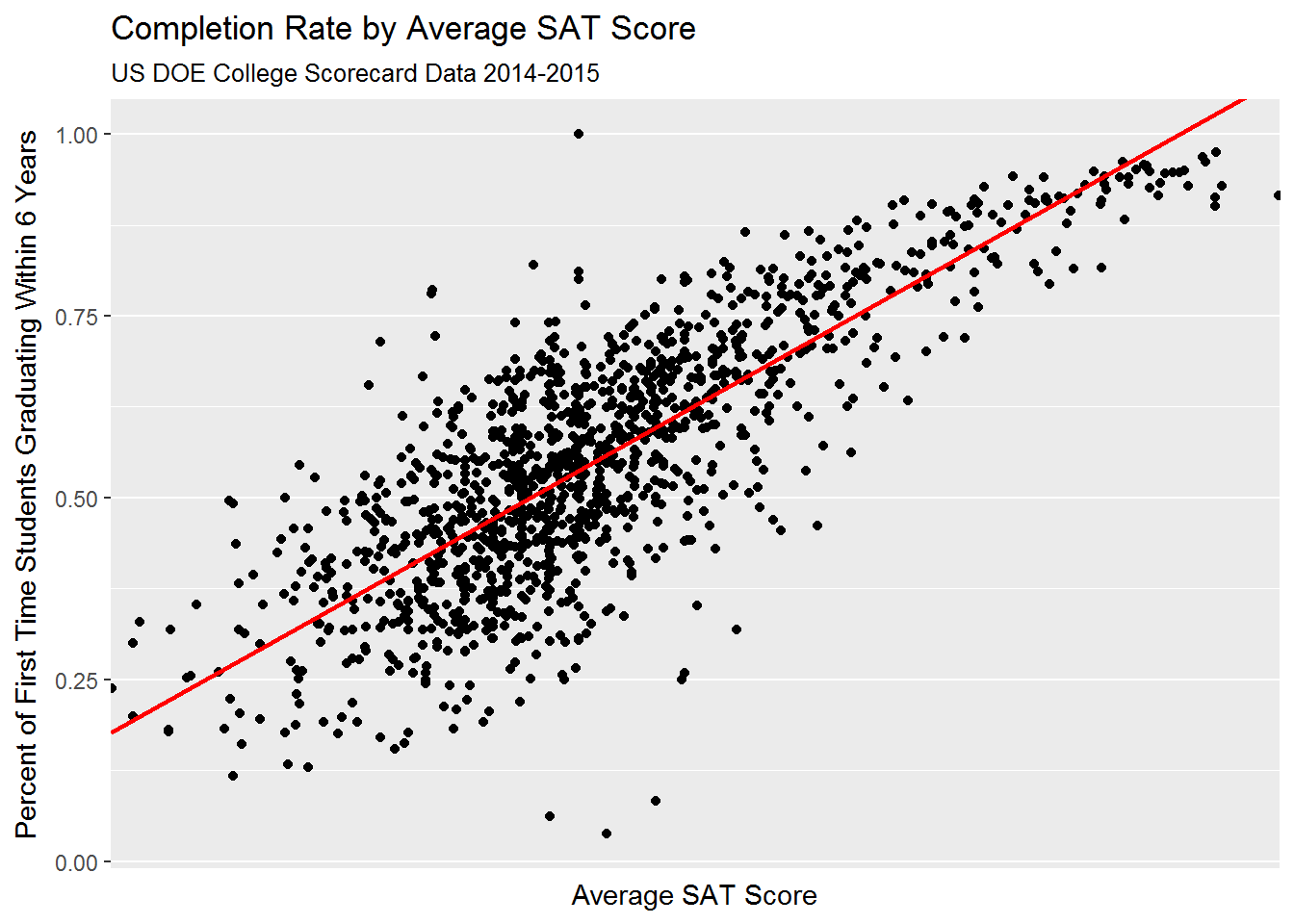
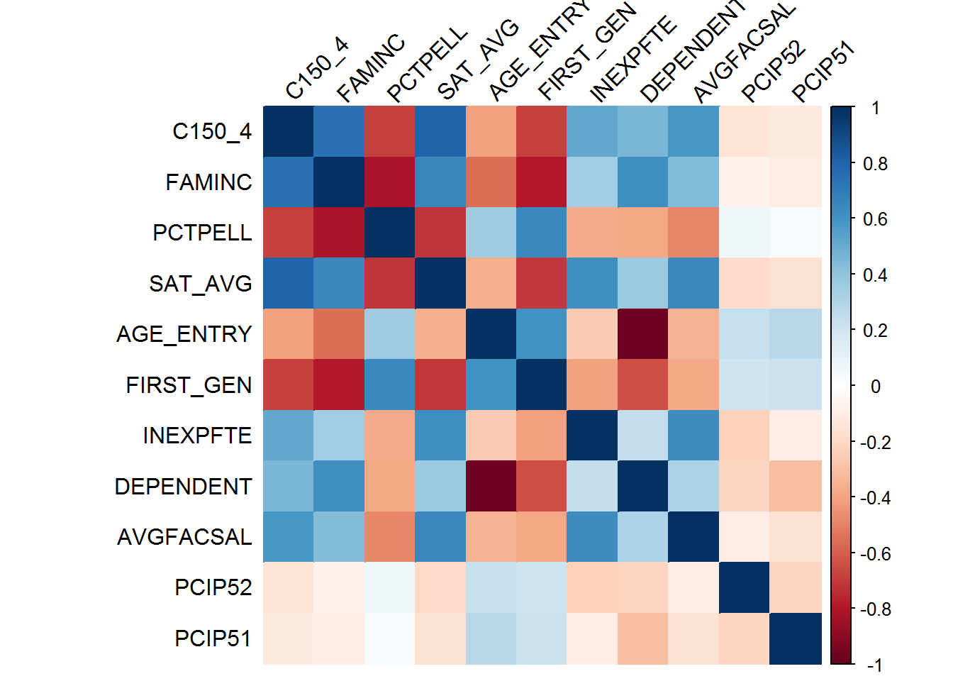
As it turns out, there is a high degree of correlation between predictors related to (1) student body’s socioeconomic background; (2) average SAT score; and (3) college’s educational expenditure:
5.2. Predict student graduation rates by college
Given the high degree of collinearity between key predictors, I opted to use Principal Component Analysis (PCA) to reduce the set of predictors to a smaller set of linearly-uncorrelated variables, while still maximizing variance of each principal component.
I used the initial regression tree to do variable selection, plugging in the predictors identified by the tree as inputs to the PCA.
This approach has several limitations: - PCA can’t handle null values. Using PCA I was only able to predict graduation rates for ~50% of colleges. Deeper analysis should account for null values using imputation or selecting predictors that have good data coverage. - PCA can only handle numeric inputs, so categorical attributes must be converted to numeric. This works well for categorical variables which are ordinal, but not so well for those which are nominal (no inherent order between levels).
library(psych)       #PCA package
library(FactoMineR)  #additional PCA analysis

#prepare pca dataset
pca.df <- data13[,cor.vars]
pca.df$C150_4 <- NULL
pca.df <- as.data.frame(lapply(pca.df , as.numeric))

#train pca
pca.rotate = principal(pca.df, nfactors=3, rotate = "varimax")

#apply pca scores
pca.scores = as.data.frame(pca.rotate$scores)
pca.df <- cbind(pca.df, pca.scores, C150_4=data13$C150_4)

#linear regression using principal components
pca.lm = lm(C150_4~RC1+RC2+RC3, data=pca.df)
summary(pca.lm)
##
## Call:
## lm(formula = C150_4 ~ RC1 + RC2 + RC3, data = pca.df)
##
## Residuals:
## Min 1Q Median 3Q Max
## -0.44221 -0.05546 0.00234 0.05771 0.51543
##
## Coefficients:
## Estimate Std. Error t value Pr(>|t|)
## (Intercept) 0.472161 0.003412 138.392 <2e-16 ***
## RC1 0.153575 0.002917 52.644 <2e-16 ***
## RC2 0.005700 0.003595 1.585 0.113
## RC3 -0.079445 0.004135 -19.211 <2e-16 ***
## ---
## Signif. codes: 0 '***' 0.001 '**' 0.01 '*' 0.05 '.' 0.1 ' ' 1
##
## Residual standard error: 0.0945 on 1298 degrees of freedom
## (1146 observations deleted due to missingness)
## Multiple R-squared: 0.6845, Adjusted R-squared: 0.6837
## F-statistic: 938.6 on 3 and 1298 DF, p-value: < 2.2e-16#Note the 1146 obs deleted due to missing values5.2a. Evaluate model results
Ultimately the PCA linear regression approach outperformed the simple regression tree trained previously.
However, this could be due to the fact that the PCA linear model is trained only on the subset of schools which report average SAT scores (roughly half the dataset), and when AVG_SAT is excluded from the PCA model, model MSE jumps and is closer to the regression tree error rate.
PCA linear model mean squared error (MSE) on test data:
## [1] 0.008997365Regression tree mean squared error (MSE) on test data:
## [1] 0.02325999Baseline for comparison - average graduation rate among colleges in test data:
## [1] 0.4779574Examine residuals - which schools are the top over/underperformers for graduation rate compared to my prediction?
Overperforming colleges are likely to be religiously affiliated private non-profit schools. Several are health/nursing focused, and many have a high percentage of female students.
##                                                    INSTNM C150_4 CONTROL
## 2855    The Christ College of Nursing and Health Sciences 0.7857       2
## 1733                      College of Our Lady of the Elms 0.7811       2
## 2888 Good Samaritan College of Nursing and Health Science 0.7143       2
## 2151                     Bryan College of Health Sciences 0.8000       2
## 3126                       Northwest Christian University 0.6625       2
## 1170                               Bethel College-Indiana 0.6983       2
## 423                         Mount Saint Mary's University 0.6550       2
## 331                             Fresno Pacific University 0.6327       2
## 1637                                  Bay Path University 0.6319       2
## 3197                                  Cedar Crest College 0.6907       2
##      RELAFFIL_IND    FEMALE     resid
## 2855            0 0.9047619 0.3698549
## 1733            1 0.7703180 0.3628841
## 2888            1 0.9379845 0.3118155
## 2151            0 0.8977273 0.2997813
## 3126            1 0.6088154 0.2686893
## 1170            1 0.6677890 0.2612087
## 423             1 0.9270705 0.2543667
## 331             1 0.7465668 0.2465729
## 1637            0        NA 0.2443710
## 3197            0 0.9345088 0.2434338
Underperforming colleges are a mix of public and private non-profit schools. There seems to be some geographic concentration in the southeast/
##                                                INSTNM C150_4 CONTROL
## 3759                               Paul Quinn College 0.0380       2
## 4094 West Virginia University Institute of Technology 0.1921       1
## 6948       Pennsylvania State University-World Campus 0.2500       1
## 945                          Truett-McConnell College 0.2216       2
## 9                     Auburn University at Montgomery 0.2194       1
## 1193  Indiana University-Purdue University-Fort Wayne 0.2640       1
## 888                        College of Coastal Georgia 0.1547       1
## 862              Abraham Baldwin Agricultural College 0.1618       1
## 7082                               Augusta University 0.3030       1
## 1232           Purdue University-North Central Campus 0.2415       1
##      STABBR      resid
## 3759     TX -0.3158816
## 4094     WV -0.3118111
## 6948     PA -0.2401925
## 945      GA -0.2399651
## 9        AL -0.2367177
## 1193     IN -0.2326425
## 888      GA -0.2292820
## 862      GA -0.2282257
## 7082     GA -0.2261134
## 1232     IN -0.2241535
To address the patterns observed in the residuals, I tried including religious affiliation and region into the PCA linear regression model, but these attributes did not improve model fit. It’s possible that: - Only certain kinds of religious schools are associated with overperformance. Or, there could be an interaction between religious affiliation and healthcare-focused schools. - The geographic relationship may be at the state level rather than at the regional level. Or, it could be that the region definition could be changed to better reflect certain underperforming regions (e.g. “Appalachian Region” vs. Mid-Atlantic and Southeast).
Infographic